Hidden Markov Models are an excellent way to predict the upcoming steps of a Markovian Process, a stochastic process in which future and past states are independent conditional upon the present state, which contains hidden states. The properties of the Hidden Markov Model make it especially useful in time based pattern recognition and reinforcement learning.

Hidden Markov Models

A Hidden Markov Model refers to a probabilistic generative model in which there are certain hidden states \(Z\) which are producing the observable results \(X\). The name derives from the fact that \(Z\) is a hidden state and that \(Z\) is supposed to transition from one hidden state to another using the form of a first order Markov Chain. Hence \(\textit{Hidden Markov}\) Model.

Some details of the HMMs are presented. Let \(\mathbf{X}=\{x_1,...,x_n\}\) represent the observed values for all steps \(n\), \(\mathbf{Z}=\{z_1,...,z_n\}\) the hidden state for each step, and \(\mathbf{\Theta}=\{\pi,A,\phi\}\) the model parameters. The joint distribution of the HMM can be represented as:

\[p(\mathbf{X},\mathbf{Z}|\mathbf{\Theta})=p(z_1|\pi)\left[\prod_{n=2}^Np(z_n|z_{n-1}, A)\right]\prod_{n-1}^Np(x_n|z_n,\phi)\]

The probability of moving from one hidden state \(j\) to hidden state \(k\) can also be represented.

\[A_{jk}\equiv p(z_{n,k}=1|z_{n-1,j},j=1)\quad \sum_k A_{jk}=1\]

The parameters are estimated via an application of the EM algorithm. Once the parameters are known, the state variables need to be estimated as well. They can be estimated through the application of the Maximum A Posteriori (MAP).

\[\hat{z}_1^n=\;{\tiny\begin{matrix}\\ \normalsize \text{argmax} \\ ^{\scriptsize z_1^n}\end{matrix}}\: p(z_1^n|x_1^n)\]

\[\hat{z}_1^n=\;{\tiny\begin{matrix}\\ \normalsize \text{argmax} \\ ^{\scriptsize z_1^n}\end{matrix}}\: log(p(z_1^n,x_1^n))\]

This is generally solved with the Viterbi algorithm.

Application

This is an extension of the dataset imputed in the Missing Values post.

Moving onto the presentation of the computed HMMs: normally the trajectories being tested should be normalized before fitting the HMM, but as the data given was already normalized, this step was able to be passed over. Utilizing the \(\texttt{python}\) library \(\texttt{hmmlearn}\) a Gaussian HMM was fit to the data and the results coming from this were analyzed.

Five-fold cross validation was used to test the validity for the HMM using different numbers of hidden states. As the attempt is to infer periods of crises from the data, it does not add much to the ability for quick inference to have too many states. This could have changed though dependent upon the results from the cross validation. The HMM was tested with different states which were set equal to \([2, 3, 4, 5]\). The results from these five different states on the testing and training data are shown in the figure below. The score therein represents the log-likelihood of that particular sequence when being tested.

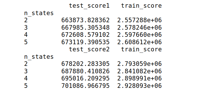
As can be noticed by the results shown in the figure above, there is not significant differences in the test scores from the various number of states. This leads one to believe that they are all likely to be suitable for identification, and there is not much return on increasing the number of hidden states especially since increased number of hidden states leads to more expensive computations.

One way to test the fits beyond using just the log-likelihood of the sequences is by using the Akaike and Bayesian Information Criteria.

\[AIC=-2log(L)+2p\]

\[BIC= -2log(L)+plog(T)\]

Where \(p\) is equal to the parameters estimated, \(Log(L)\) is equal to the log-likelihood of sequences of the model, and \(T\) is equal to the number of observations.

The idea is to select the BIC and AIC which are the lowest as it helps keep a good combination between goodness of fit and simplicity. The AICs and BICs calculated are shown in the following figure.

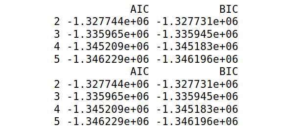
Once again the idea is to select the AIC and BIC values which are the lowest, but it is also evident that the values are not changing significantly when moving from one state to the other.

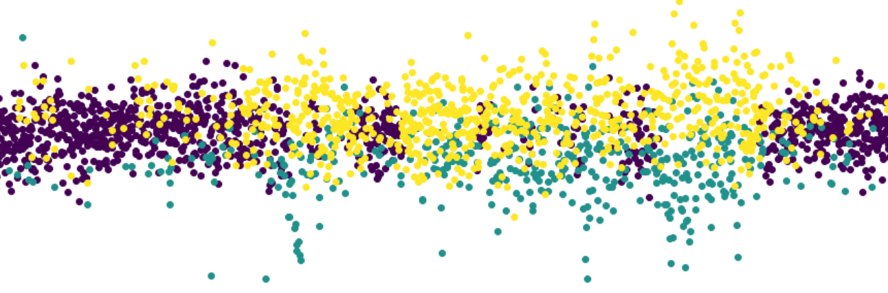
Since there were no strong specifics for using any specific number of states, different values of hidden states were analyzed along with their ability to infer states from the model. First a graph demonstrating when the states were on or off were analyzed. The next few figures demonstrate the results with varying numbers of hidden components.

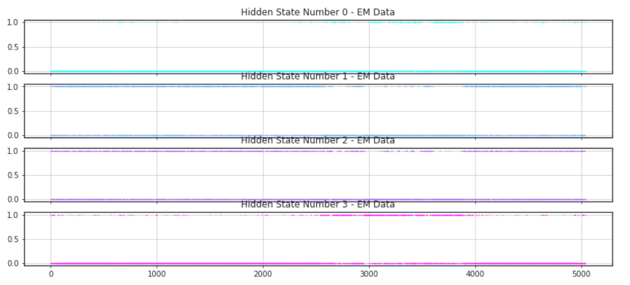
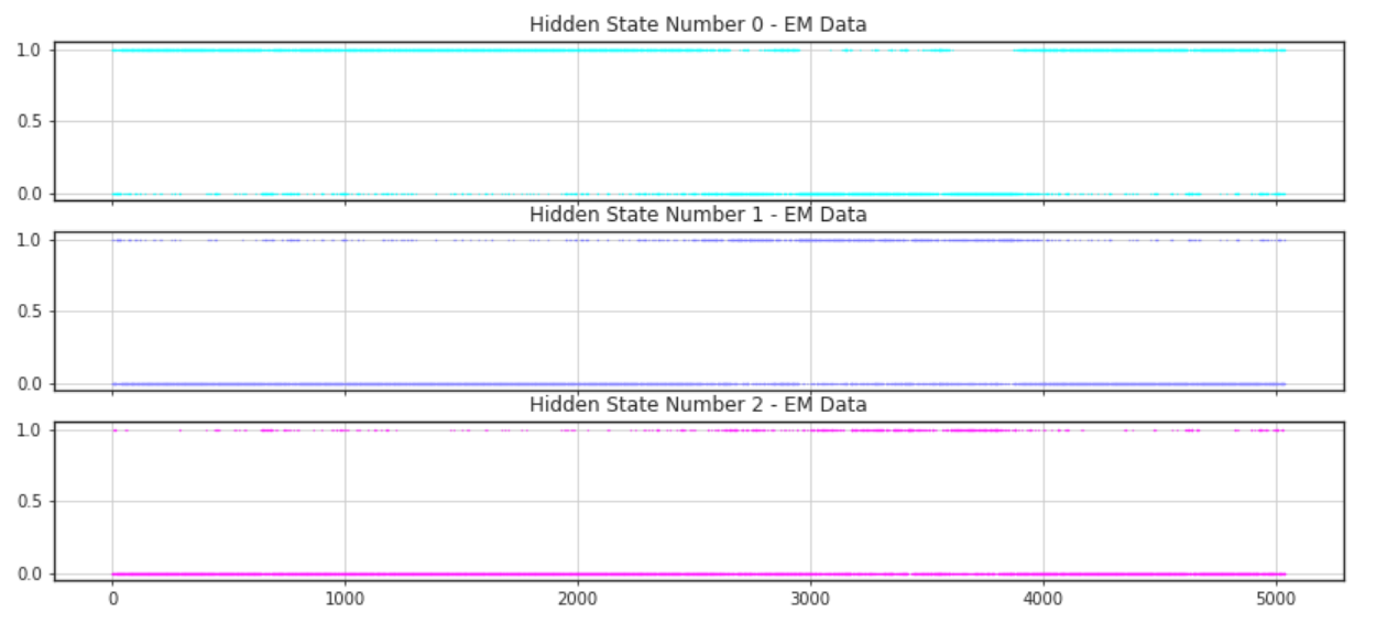
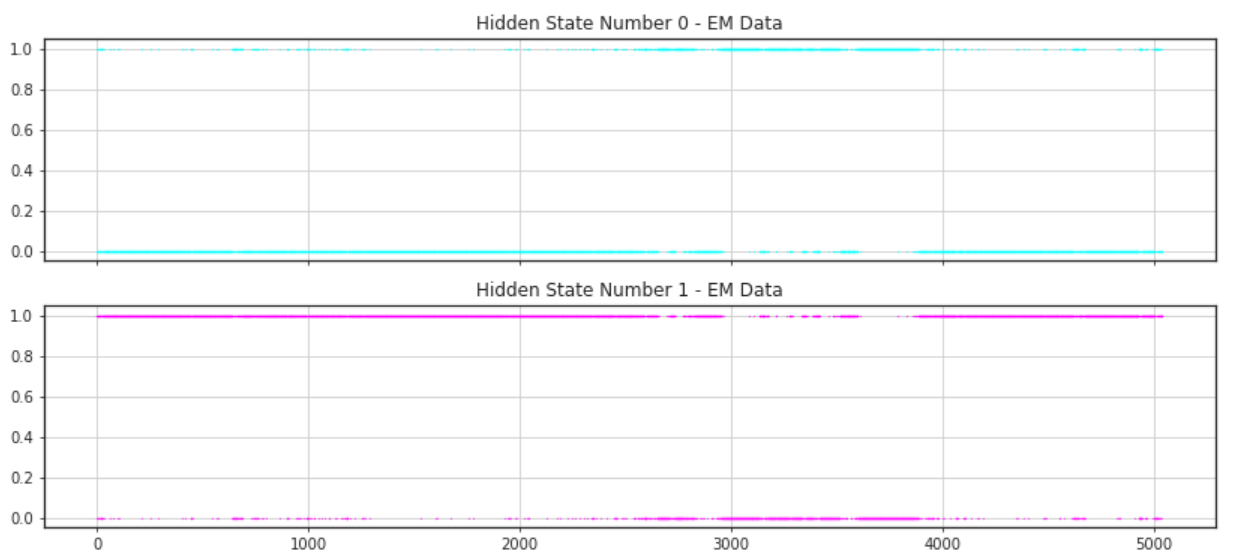
As can be noticed there seems to be a difficulty in identifying where the states are dominant when the number of hidden states is equal to four. However, there does seem to be a more common trend among the graphs representing three and two hidden states. For both of these there seem to be one hidden component which is generally active. This seems like a good target to decide to use as a general marker for the general state of the market. The other hidden states of these two graphs seem to identify a similar area as well. This may be because there is one hidden state which is in between the other two and is simply identifying areas where there is less variance.

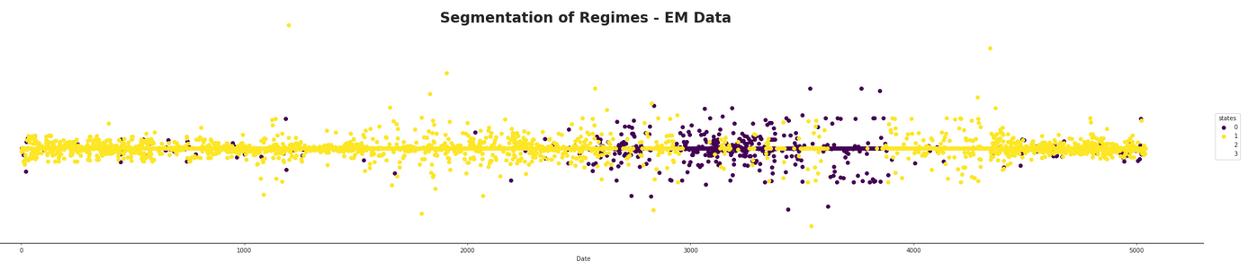
Then some different indexes were tested out and marked over time according to their set number of components. The following figure demonstrates this for a component (ADP) which has an average number of incoming edges from the DAG. This would lead us to assume that it will follow more generally from the model.

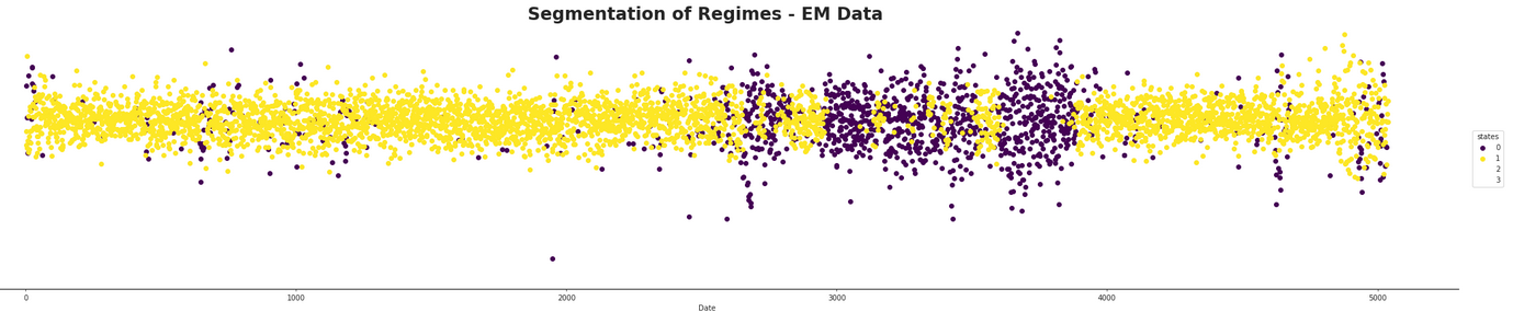
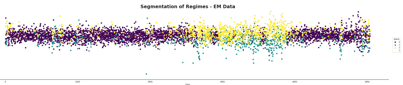
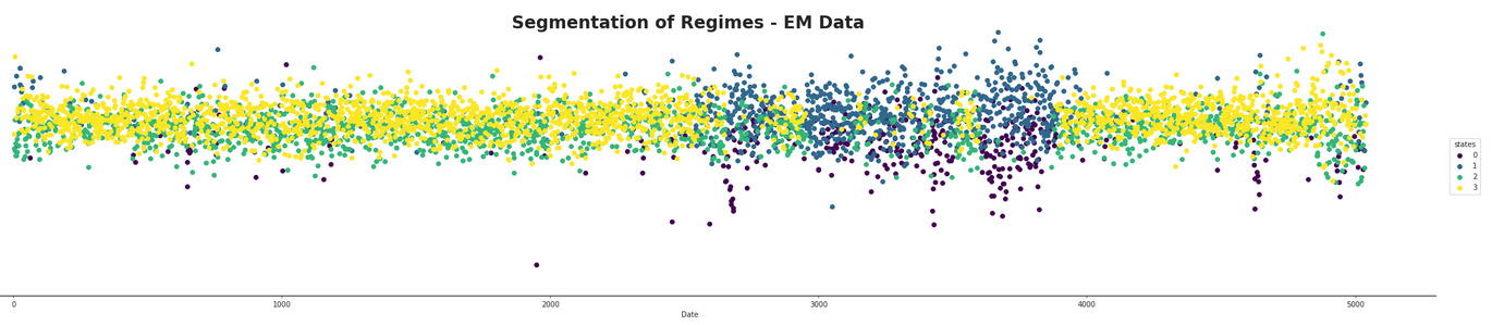
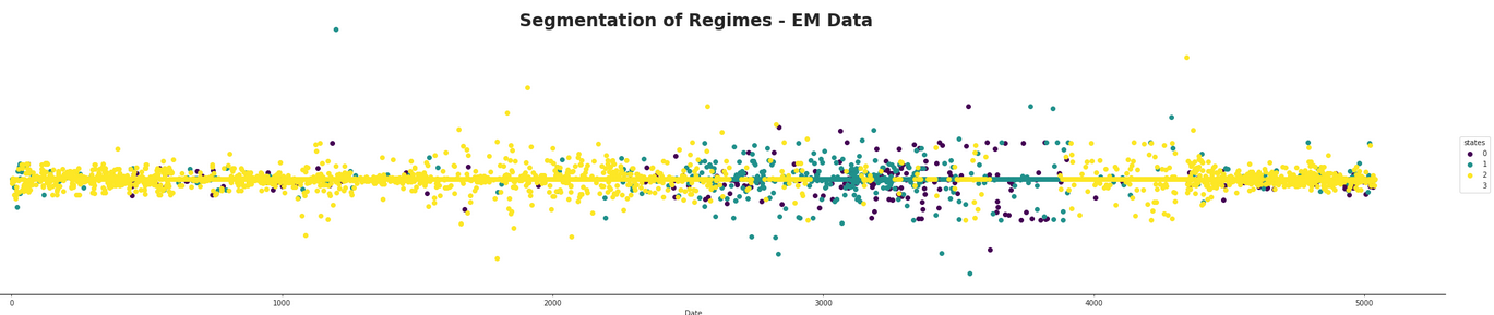
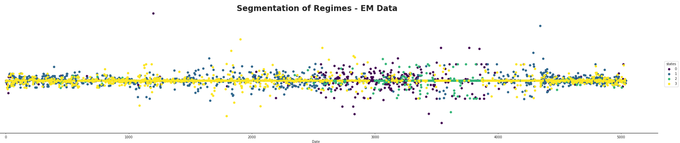
As speculated before, there seems to be a dominant state which is likely the normal market state. At first glance, it is hard to infer much from the HMM with four states as it appears to be much more mixed than the other two. It seems that both the two and three hidden component segmentations are capturing the same data, but that the three component one seems to split between one component selecting the normal state, one capturing areas where the returns appear to be better than average, and the third state capturing areas where the returns appear to be doing worse than average. They both appear to be capturing areas of high volatility in the market and furthermore they appear to be quite mixed in with each other. The following figure shows this mixing with a finer detail.

It appears that there is the possibility of anticipating high areas of volatility, but quite difficult to say whether or not the volatility will be in a positive or negative direction for a long time period. It could be possible that using short term hidden state estimation could allow for gaining a slight edge on the market. This is tested later in this section. The high volatility likely means the market is more in a state of chaos, with larger losses and larger gains occurring in succession with each other. The areas which are dominated by the hidden states not pertaining to the normal state of the market definitely seem to be states of, if not crisis, at least high uncertainty for investors.

Next a index with no dependencies on the DAG was modeled. This was the ANF index.

As what could be suspected, the hidden states here seem to have a less effective role in predicting the states of volatility. The states don't correspond as nicely with the data as in the ADP index and actually do not appear to give very much helpful information at all. One interesting part of this index is there seems to be much less variability when compared to the other ADP index.

When comparing the results given by the HMM, it was noticed that the period of high volatility noted in the chart seemed to correspond well with the high variability in the French Market noted between 1998-2002 when the market enthusiastically ran into a bull market and then as quickly slumped down. It would have been very interesting to have data from the time period relating to the next big crash which came in 2008, but it was not available. It can be noted that by the end of this time period, it does not appear that there are any clear warning signs of the impending crash.

Finally the HMM model could be utilized to predict the next hidden state in the time series. The idea in computing the next hidden state is to find \(P(Z^{t+1})\). Due to the memoryless property of Markov chains the variable for the next step only depends on the posterior probabilities of the hidden states of the last step and the transition matrix. Therefore the next state can be seen as the following:

Experiments with predicting the next hidden state came up with the following results. The hidden state was able to be predicted for the next time period, but after a few time-steps the predicted value would generally converge towards the "normal" state. This was likely due to the very dominant centered structure of the data. Thus it appears that the HMM should only be used to forecast hidden states which are close in the future. A possible extension to performing prediction in a more robust manner could be using the EM algorithm to predict future values and then predict the hidden states on this fore-casted data.