Having a large collection of data is always a wonderful thing because it allows inferences and dependencies to be gleaned. The problem with great amounts of data is the fact that using all of this data can lead to both overfitting and being struck by the curse of dimensionality. In this post I go over a basic approach to dimension reduction and some reasons why it is so important.

The Curse of Dimensionality

The important thing to realize regarding dimensionality is that the feature space needed increases exponentially with additional features. As an example, 10 data points in one dimension can be represented as 10 points on a line, 10 data points in two dimensions is equivalent to \(10^2\), and more generally the feature space necessary for \(n\) dimensions is represented as \(10^n\). This creates unnecessary sparsity and an obvious way to combat this is to minimize the amount of features needed to generalize the data effectively. This is what is known as dimension reduction.

Dimension Reduction

Dimension Reduction is important because it avoids the curse of dimensionality, helps machine learning models avoid overfitting, and improves the run time of algorithms. There are many methods used for implementing dimension reduction, but the most typical one is called PCA (Principal Component Analysis).

PCA

PCA is a linear technique, although techniques such as using the kernel trick to produce kernel PCA provide a good method for nonlinear problems, that preserves the maximum amount of variance while mapping the data to a lower dimensional feature space. It provides for an easy method in dropping features which add the least variance to the problem.

Consider a \(m \times n\), \(m\) dimensional data and \(n\) observations, data matrix \(\mathbf{X}\). A brief discussion of how to apply PCA to this datset is as follows (note that much of the theory is passed over):

1. Compute the covariance matrix \(\mathbf{S}\)
   • find the mean vector \(\mathbf{\mu} = \frac{1}{n}(\mathbf{x}\_1+...+\mathbf{x}\_n)\)
   • shift the data in \(\mathbb{R}^m\) to produce \(\mathbf{B}= [\mathbf{x}_1-\mathbf{\mu}|...|\mathbf{x}_n-\mathbf{\mu}]\)
   • \(\mathbf{S} = \frac{1}{n-1}\mathbf{B}\mathbf{B}^T\)
     • in practice \(\frac{1}{n-1}\) is often discarded
2. Find the eigenvalues \(\lambda_1\),...,\(\lambda_m\) of \(\mathbf{S}\) arranged from largest to smallest along with orthonormal eigenvectors \(\mathbf{v}_1\),...,\(\mathbf{v}_m\)
3. Variance produced by each variable can be reproduced by divided the eigenvalue by the trace of \(\mathbf{S}\)
   • The ordering of the eigenvalues from largest to smallest allow us to easily observe the amount of variance the principal directions account for.
     • Consider a three dimensional data set with very little variance in the \(\vec{z}\) axis, but a fair amount in the \(\vec{x}\) and \(\vec{y}\) axes. The main principal directions would be on the \(\vec{x}\) and \(\vec{y}\) axes.
   • It is up to the researcher to decide which eigenvalues to drop, but the smallest eigenvalues relate to the smallest principle components.
   • The eigenvectors describe the weight, or shape, of each variable upon the corresponding principle direction.
     • This can be used to intuitively see which variables have less of an effect, whether they are a positive or negative influence, etc.

As mentioned previously, applying the kernel trick along with PCA is a method to reduce dimensionality of nonlinear data.

Application

This is an attempt to apply PCA to the datset imputed from the Missing Values post and worked upon in the Dependency Inference post.

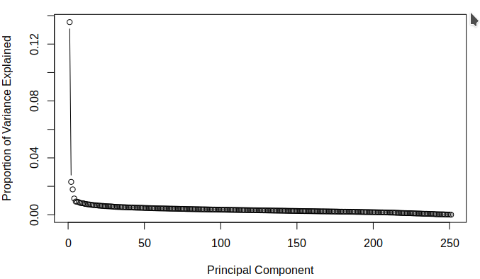
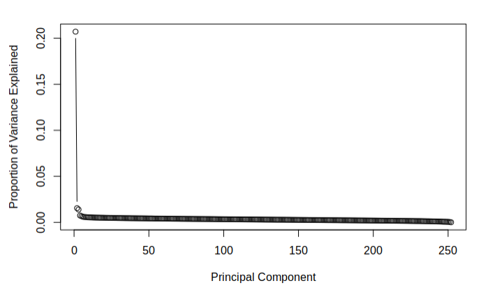
The purpose of attempting dimension reduction was to attempt to lower the dimensionality of the model and discover if there were any components of the \(\texttt{SBF250}\) which did not add much information for the model to learn from. The aim was to discover which principle components contain the most variance. This is done easily by dividing the variance of each component by the sum of all the components' variances. The following figures demonstrate the proportion of total variance explained by each component starting from the largest and going to the smallest for each of the calculated datasets.

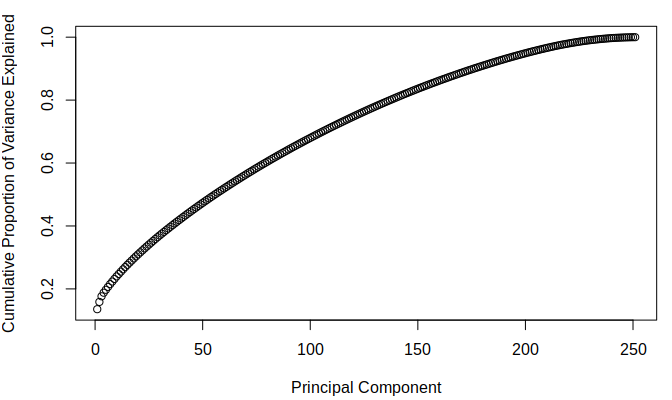
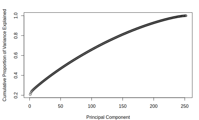
The below figures demonstrate the cumulative proportion of variance explained from each dataset. From the graphs it is rather easy to see that there is not much candidacy for principal components which can be easily removed as it seems that most of them are quite similar in value. The tail ends could be removed, but it is not a great effect upon the large dimensionality of the data. Since the data is already very high dimensional, it does not make much sense to remove only a few parameters of the data and thus it was decided that the full data set would be used while moving on. It was interesting to note that there was not much difference in the principle components of the two different imputed sets.

Resources

-Jauregui, Jeff. “Principal Component Analysis with Linear Algebra.” Jeff Jauregui, Union Math, Union College, 2013, www.math.union.edu/~jaureguj/.