Data mining and exploratory data analysis are both key weapons in any data science toolbox. An important component of exploring data is determining dependencies and conditional independence relations so as to better be able to understand the underlying structure of data.

Dependency Inference

Probabilistic Graphical Models can be useful because of the fact that they allow one to easily infer dependencies and conditional independence relations in a visual manner. PGMs follow the Global Markov Property which can be stated as follows: Given any three subsets of the PGM, in this case \(\mathbf{X}_A\), \(\mathbf{X}_B\), and \(\mathbf{X}_C\), \(\mathbf{X}_A\perp\!\!\!\perp|\mathbf{X}_B|\mathbf{X}_C \Leftrightarrow \mathbf{X}_C\) separates \(\mathbf{X}_A\) from \(\mathbf{X}_B\) in the moral graph of the subgraph induced by these three disjoint subsets. This means that global conditional independence relations are obtained.

In the Bayesian setting it is possible to have consistent PGM estimation using the maximization of the log of the posterior. Supposing there is a \((\mathcal{G},\theta)\) representing a probabilistic graphical model with \(\mathcal{G}\) representing the structure of the graph and \(\theta \in \Theta\) the probability model parameter. Let the prior probability distributions \(\pi\) for \(\mathcal{G}\) and \(\theta\) be specified as dictated by their belonging to the Bayesian paradigm. A Bayesian scoring function constructed for a sample \(D_n\) of size \(n\) is represented as \(S(\mathcal{G}|D_n)\). This also includes the function \(\mathcal{L}(\mathcal{G}|D_n)\) which represents the marginal likelihood of \(\mathcal{G}\) and wherein \(\mathcal{L}(\mathcal{G},\theta|D_n)\) is the usual likelihood of \((\mathcal{G},\theta)\).

\[S(\mathcal{G}|D*n)=log\pi(\mathcal{G}) + log \mathcal{L}(\mathcal{G}|D_n)\]

\[\mathcal{L}(\mathcal{G}|D_n)=\int_{\theta \in \Theta}\mathcal{L}(\mathcal{G},\theta|D_n)\pi(\theta)d\theta\]

The best estimator of the PGM is a natural result from the natural consistent directed PGM chosen when the scoring function \(S(\mathcal{G}|D_n)\) is maximized. This function is very difficult to maximize and falls into the realm of NP-hard problems which means that generally algorithms are utilized in order to get a nice approximation of the true maximal PGM.

The algorithm chosen for use in this report is one set forth by Chickering in 2002. This method is called the Greedy Equivalence Search algorithm and was selected due to the fact that other attempted algorithms did not seem to come to a nice convergence when running them, possibly due to the high dimensionality of the data.

The idea behind the GES algorithm is that given that the generative distribution has a perfect map in the Directed Acrylic Graph defined over the observable data then there must be a sparse search space to which a greedy search algorithm can be applied in order to find that generative structure. This idea is referred to as Meek's Conjecture and was unproven for a number of years despite making what seemed like good sense.

Meek's Conjecture can be stated as the following: there are \(\mathcal{H}\) and \(\mathcal{G}\) which are Directed Acrylic Graphs with \(\mathcal{H}\) being the independence map of the graph \(\mathcal{G}\). This means that any independence implied by either structure also implies independence in the other structure, provided that the conjecture is true. The implication from this is that there are a finite number of edge additions and covered edge reversals which can be applied to \(\mathcal{G}\) provided that after each step \(\mathcal{G}\) remains a DAG and \(\mathcal{H}\) remains the independence map of \(\mathcal{G}\) and that after all steps are covered that \(\mathcal{G} = \mathcal{H}\). Meek's Conjecture was proved true by Chickering and thus the GES was created.

The GES algorithm has two main steps. The algorithm initialization is the state where the DAG has no edges and thus has the equivalence class which corresponds to no dependence relations among any of the variables. The first phase then moves from the initialization forward until a local maximum of the DAG has been reached. The second phase then consists of moving from the local maximum found in phase one in the backwards direction to another local maximum. So the algorithm consists of simply iterating forward and backward until convergence.

The following theorem by Chickering describes how the GES algorithm leads to a solution for PGM estimation.

Theorem 1 (Chickering 2002) Let \(\mathcal{G}\) and \(\mathcal{H}\) be any pair of DAGs such that \(\mathcal{G} \le \mathcal{H}\), let \(r\) be the number of edges in \(\mathcal{H}\) that have opposite orientation in \(\mathcal{G}\), and let \(a\) be the number of edges in \(\mathcal{H}\) that do not exist in either orientation in \(\mathcal{G}\). There exists a sequence of at most \(r+2a\) distinct edge reversals and additions in \(\mathcal{G}\) with the following properties:

1. Each edge reversed is a covered edge
2. After each reversal and addition \(\mathcal{G}\) is a DAG and \(\mathcal{G} \le \mathcal{H}\)
3. After all reversals and additions \(\mathcal{G} = \mathcal{H}\)

Application

This section looks at data for which missing values were imputed using the methods outlined in the Missing Values post. This dataset contains 250 columns pertaining to the 250 different companies of the SBF250 French stock market index and 5039 observations of the normalized daily returns of these companies. The data is assumed to follow a multi-variate normal distribution.

Since the data is large with many variables, it was not really possible to visualize in a helpful manner the Directed Acrylic Graph which helps represent the dependencies across the entire dataset of the SBF250. Rather than producing a DAG which didn't help with analysis the numbers of nodes and edges going into each node were analyzed.

Analyzing the numbers of incoming edges proved very interesting. It seems that both methods of missing value imputation managed to produce DAGs which contained the same number of edges incoming into each node. The values incoming are represented in the two following histograms.

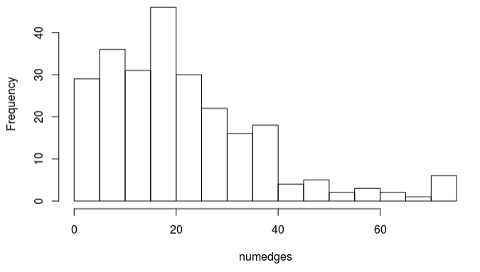
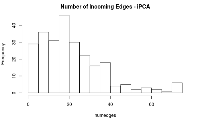
Furthermore, it appeared that there were two nodes which did not have any incoming nodes at all, with the average node having 21.5 incoming edges, and the node with the most edges having 75 incoming edges. The incoming number of edges appears to take on a right skewed distribution with the peak right around 20 edges. This means that in general the model was very highly connected, with only the two independent nodes. This makes sense in the fact that it empirically makes sense from an economics perspective that the market index will stay more tightly grouped and is more of a indication as to how the general economy is doing rather than a completely independent event. It also makes sense when realizing that the imputed datasets both were imputed with the importance of maintaining the relationships inherent in the covariance structure.

Resources

• D. Chickering. Optimal Structure Identification With Greedy Search. Journal of Machine Learning Research, (3):507–554, 2002.
• J.-B. Durand. Lecture notes in fundamentals of probabilistic data mining, January 2018